Statistics overview

This guide summarizes the core ideas from the statistics lessons: descriptive statistics, common probability distributions, and how to choose a statistical test. For statistical test selection, use the quick guide first, then refer to the complete table for edge cases and more specific scenarios.

1. Common descriptive statistics

Descriptive statistics summarize and describe the main features of a dataset. They are divided into three main categories based on what aspect of the data they measure.

1.1. Measures of central tendency, spread, and shape

Category	Statistic	Description	Formula / Calculation	When to use	Python implementation
Central tendency	Mean (μ or x̄)	Average of all values; sum divided by count	μ = Σx / n	Symmetric distributions without outliers	np.mean(data) or data.mean()
	Median	Middle value when data is ordered; 50th percentile	Middle value or average of two middle values	Skewed distributions or data with outliers	np.median(data) or data.median()
	Mode	Most frequently occurring value(s)	Value with highest frequency	Categorical data or multimodal distributions	statistics.mode(data) or data.mode()
	Trimmed mean	Mean after removing extreme values (for example top/bottom 5%)	Mean of remaining values after trimming	Data with outliers but want mean-like measure	scipy.stats.trim_mean(data, 0.05)
Spread	Range	Difference between maximum and minimum values	Range = max - min	Quick measure of spread; sensitive to outliers	np.ptp(data) or max(data) - min(data)
	Variance (σ² or s²)	Average squared deviation from the mean	σ² = Σ(x - μ)² / n	Understanding variability; basis for other stats	np.var(data) or data.var()
	Standard deviation (σ or s)	Square root of variance; typical distance from mean	σ = √(Σ(x - μ)² / n)	Most common spread measure; same units as data	np.std(data) or data.std()
	Interquartile range (IQR)	Difference between 75th and 25th percentiles	IQR = Q3 - Q1	Robust to outliers; used in boxplots	scipy.stats.iqr(data) or data.quantile(0.75) - data.quantile(0.25)
	Mean absolute deviation (MAD)	Average absolute deviation from the mean	MAD = Σ|x - μ| / n	Less sensitive to outliers than variance	np.mean(np.abs(data - np.mean(data)))
	Coefficient of variation (CV)	Relative standard deviation (standardized measure)	CV = (σ / μ) × 100%	Comparing variability across different scales	(np.std(data) / np.mean(data)) * 100
Shape	Skewness	Measure of asymmetry in the distribution	Positive: right tail; Negative: left tail; 0: symmetric	Assessing distribution symmetry	scipy.stats.skew(data) or data.skew()
	Kurtosis	Measure of tailedness (outlier propensity)	Positive: heavy tails; Negative: light tails; 0: normal	Identifying presence of outliers	scipy.stats.kurtosis(data) or data.kurtosis()

1.2. Interpretation guidelines

Central tendency

• Mean = Median = Mode: Perfectly symmetric distribution
• Mean > Median: Right-skewed (positive skew) distribution
• Mean < Median: Left-skewed (negative skew) distribution

Spread

• Low variance/SD: Data points cluster closely around the mean
• High variance/SD: Data points are widely dispersed
• IQR: Contains the middle 50% of the data
• CV < 15%: Low variability; CV > 30%: High variability

Shape

• Skewness:

  • Between -0.5 and 0.5: Approximately symmetric
  • Between -1 and -0.5 or 0.5 and 1: Moderately skewed
  • Less than -1 or greater than 1: Highly skewed

• Kurtosis (Excess Kurtosis):

  • Approximately 0: Normal distribution
  • Greater than 0: Heavy tails, more outliers
  • Less than 0: Light tails, fewer outliers

1.3. Choosing the right statistic

1. For symmetric data without outliers: Use mean and standard deviation
2. For skewed data or data with outliers: Use median and IQR
3. For comparing variability across different scales: Use coefficient of variation
4. For understanding distribution shape: Calculate skewness and kurtosis
5. For categorical data: Use mode and frequency tables

1.4. Important notes

• Always visualize your data (histograms, boxplots, Q-Q plots) before choosing statistics
• Report multiple measures to give a complete picture of your data
• Consider the context and purpose of your analysis when selecting statistics
• Remember that descriptive statistics can be misleading without understanding the underlying distribution

2. Statistical test selection guide

Before selecting a test, check the data type, distribution shape, and whether the samples are independent.

The tests listed below cannot be used with nominal data as the dependent variable. Choosing the correct statistical test and plotting data effectively depends on the data's statistical type. See the Wikipedia article Statistical data type for more information.

The tests below come in two flavors that differ in assumptions. Parametric tests (t-test, F-test) make assumptions about the population's distribution and parameters, non-parametric tests (Mann-Whitney, Kruskal–Wallis) do not. Parametric vs non-parametric is a useful distinction when thinking about statistical tests and models. See Parametric and Nonparametric: Demystifying the Terms.

2.1. Most common/useful tests

2.1.1. Student's t-test

• Use this test for comparing two groups.
• Wikipedia article: Student's t-test
• SciPy.stats implementation: ttest_ind()

Notes: Tests wether the difference between two groups is significant or not. Assumes that the data from which the samples were drawn is normally distributed and the samples have the same variance. If this is not true, see the Mann-Whitney U test, below.

2.1.2. ANOVA (also known as the F-test)

• Use this test for comparing multiple groups.
• Wikipedia article: F-test
• SciPy.stats implementation: f_oneway()

Notes: Tests whether or not one or more of the group means are different from the others. Assumes the data was drawn from a normally distributed population. If this is not true, see the Kruskal–Wallis test, below. Determining which sample(s) is/are different requires further analysis (see Tukey's range test).

2.1.3. Mann-Whitney U test

• Use this test for comparing two groups that are not normally distributed.
• Wikipedia article: Mann–Whitney U test
• SciPy.stats implementation: mannwhitneyu()

Notes: Uses the rank order of observations to test for difference between two groups. Data must be at least ordinal (larger or smaller has a clear meaning) and assumes that the shapes of the sample distributions are similar. If you decide not to use this test because the sample distributions look very different, you have your answer already. For completeness, maybe see the Kolmogorov–Smirnov test anyway.

2.1.4. Kruskal-Wallis test (also known as ANOVA on ranks)

• Use this test for comparing two or more groups that are not normally distributed.
• Wikipedia article: Kruskal–Wallis test
• SciPy.stats implementation: kruskal()

Notes: Uses rank order of observations to test whether or not one or more groups is different from the others. Follows the similar assumptions to the Mann-Whitney U test, above.

2.5. Assumption checklist

• Verify normality when using parametric tests.
• Check whether observations are independent.
• Confirm that groups have similar variance when required.
• Use non-parametric tests when sample size is small, data are ordinal, or assumptions are not met.

2.6. Complete test table

Independent variable type	Dependent variable type	Situation	Parametric test	Non-parametric test	P-value interpretation
None	Continuous	Comparing one sample to a known value	One-sample t-test / Z-test	Wilcoxon signed-rank test	Low p-value: Sample mean significantly differs from known value
None	Continuous	Testing normality of data	Shapiro-Wilk test	Kolmogorov-Smirnov test	Low p-value: Data significantly deviates from normal distribution
None	Continuous	Comparing sample distribution to theoretical distribution	N/A	Kolmogorov-Smirnov test	Low p-value: Sample distribution differs from theoretical distribution
Categorical	Categorical	Comparing distributions of categorical variables	Chi-square test	Fisher's exact test (for small samples)	Low p-value: Observed distribution differs from expected
Categorical	Continuous	Comparing two independent groups	Independent samples t-test / Two-sample Z-test	Mann-Whitney U test (Wilcoxon rank-sum test)	Low p-value: Significant difference between the two groups
Categorical	Continuous	Comparing two paired/dependent groups	Paired t-test	Wilcoxon signed-rank test	Low p-value: Significant change between paired observations
Categorical	Continuous	Comparing three or more independent groups	One-way ANOVA	Kruskal-Wallis H test	Low p-value: At least one group differs from the others
Categorical	Continuous	Comparing three or more paired/dependent groups	Repeated measures ANOVA	Friedman test	Low p-value: Significant differences across repeated measurements
Categorical	Continuous	Testing effects of two or more factors	Two-way ANOVA / Factorial ANOVA	Scheirer-Ray-Hare test	Low p-value: Significant main effects or interaction effects
Categorical	Continuous	Comparing variances between two groups	F-test (Levene's test)	Levene's test / Fligner-Killeen test	Low p-value: Variances significantly differ between groups
Categorical	Categorical	Testing independence of two categorical variables	Chi-square test of independence	Fisher's exact test	Low p-value: Variables are dependent (not independent)
Continuous	Continuous	Testing relationship between two continuous variables	Pearson correlation	Spearman rank correlation / Kendall's tau	Low p-value: Significant correlation exists between variables

2.7. Multiple testing correction

When you run many tests, the chance of false positives increases.

• Bonferroni is the simplest and most conservative correction.
• Holm-Bonferroni is less conservative than Bonferroni.
• Benjamini-Hochberg controls the false discovery rate.
• Post-hoc tests are appropriate after ANOVA when comparing specific group pairs.

3. Common probability distributions

Probability distributions describe the likelihood of different outcomes in a random process. They are fundamental to statistical inference, hypothesis testing, and predictive modeling.

Type	Distribution	Parameters	Description	Python implementation	Distribution shape
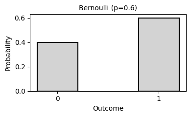
Discrete	Bernoulli	p (probability of success)	Single trial with two outcomes (success/failure)	stats.bernoulli.pmf(k, p)
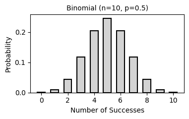
	Binomial	n (trials), p (probability)	Number of successes in n independent Bernoulli trials	stats.binom.pmf(k, n, p)
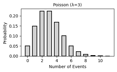
	Poisson	λ (lambda, rate)	Number of events in fixed time/space interval	stats.poisson.pmf(k, mu)
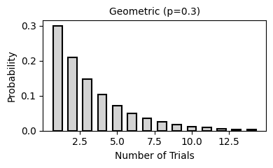
	Geometric	p (probability of success)	Number of trials until first success	stats.geom.pmf(k, p)
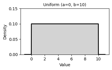
Continuous	Uniform	a (min), b (max)	All values in interval [a, b] equally likely	stats.uniform.pdf(x, a, b-a)
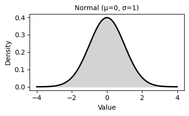
	Normal (Gaussian)	μ (mean), σ (std dev)	Symmetric bell curve; most common distribution	stats.norm.pdf(x, mu, sigma)
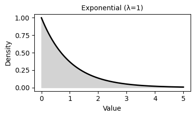
	Exponential	λ (rate)	Time between events in Poisson process	stats.expon.pdf(x, scale=1/lambda)
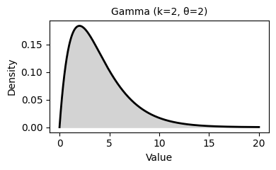
	Gamma	k (shape), θ (scale)	Generalizes exponential; sum of k exponential variables	stats.gamma.pdf(x, k, scale=theta)
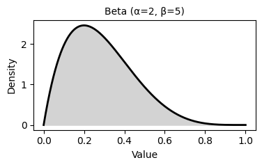
	Beta	α (alpha), β (beta)	Distribution on interval [0, 1]	stats.beta.pdf(x, alpha, beta)
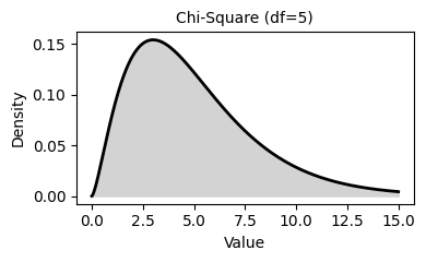
	Chi-square (χ²)	df (degrees of freedom)	Sum of squared standard normal variables	stats.chi2.pdf(x, df)
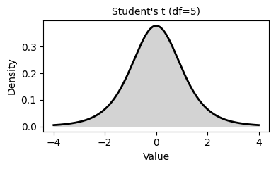
	Student's t	df (degrees of freedom)	Similar to normal but with heavier tails	stats.t.pdf(x, df)
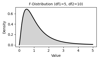
	F-distribution	df1, df2 (degrees of freedom)	Ratio of two chi-square distributions	stats.f.pdf(x, df1, df2)
	Pareto	α (shape), xₘ (scale/minimum)	Power law distribution; models 80/20 rule phenomena	stats.pareto.pdf(x, alpha, scale=xm)
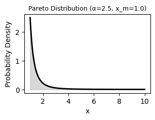