Signal Correction Pipeline: From Raw Counts to Science-Ready Data
Time to tackle the full signal correction pipeline! After understanding the timing structure and CDS basics, it’s time to implement all six preprocessing steps to turn noisy detector outputs into clean, calibrated data suitable for exoplanet analysis.
Check out the signal correction notebook on GitHub.
1. Six-Step image correction pipeline
Following the competition organizers’ guidance, here’s the complete preprocessing workflow:
- Analog-to-Digital Conversion - Convert raw detector counts to physical units
- Hot/Dead Pixel Masking - Remove problematic pixels using sigma clipping
- Linearity Correction - Apply polynomial corrections for detector non-linearity
- Dark Current Subtraction - Remove thermal background noise
- Correlated Double Sampling (CDS) - Subtract paired exposures to reduce read noise
- Flat Field Correction - Normalize pixel-to-pixel sensitivity variations
2. Step-by-step rsults
Here’s how the frames from both instruments evolve through each correction step:
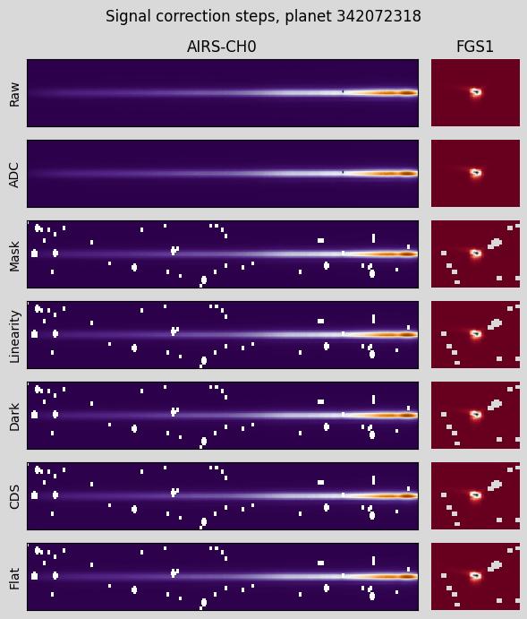
Each step addresses specific detector artifacts:
- ADC conversion transforms raw counts using gain and offset corrections
- Masking removes hot pixels (identified via sigma clipping) and known dead pixels
- Linearity correction applies polynomial fits to account for non-linear detector response
- Dark subtraction removes thermal background scaled by integration time
- CDS subtracts the short/long exposure pairs to reduce read noise
- Flat fielding normalizes pixel-to-pixel sensitivity differences
3. Transit detection
Can we still see exoplanet transits after signal correction?
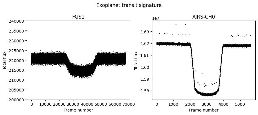
Excellent! The transit signal is clearly visible in both instruments after correction. Surprisingly, the AIRS data shows the transit even more clearly than the FGS data - apparently it’s a proper science instrument, not just an alignment camera. We are still looking in a tiny drop in signal for both instruments during this planet’s transit: ~1.5% for FGS1 and ~2.5% for AIRS-CH0.
4. Performance considerations
The full six-step pipeline works, but it’s computationally expensive. Processing one planet takes significant time, and with Kaggle’s 4-core limit, we need to think about optimization strategies:
- Refactor into a clean module - Package the preprocessing into a reusable module (maybe even deploy to PyPI for easy installation)
- Smart data reduction - Crop signals and downsample FGS data to match AIRS timing
- Parallelize where possible - Take advantage of multiple cores for batch processing
- Order of operations - Apply data reduction steps early to minimize processing overhead
5. Next steps
With the signal correction pipeline working and transits clearly visible in the processed data, the foundation is solid. The next priorities are:
- Optimize the preprocessing workflow for speed and reliability
- Implement intelligent cropping to focus on the actual signal regions
- Develop transit detection algorithms to automatically identify and extract relevant time windows
- Build the spectral extraction pipeline to turn corrected AIRS data into planetary spectra
Next up, refactor the signal preprocessing pipeline. The next day is going to feel more like engineering than science, but stay tuned - we are making progress!