Understanding Timing and CDS: Making Sense of the Axis Info
Time to dig into the timing metadata and figure out how these instruments actually work together. The axis info data turned out to be much more useful than I initially thought - it’s not about satellite alignment at all, but about the structure of the signal matrices themselves.
Check out the axis info EDA notebook on GitHub.
1. What’s in the axis info?
The axis info metadata gives us the key to understanding how the telescope data is organized:
- AIRS-CH0-axis0-h: Time index for AIRS readings (in hours, ~0.1 second resolution)
- AIRS-CH0-axis2-um: Wavelength across frames in micrometers (~1.6 μm range, high-energy IR)
- AIRS-CH0-integration_time: Detector accumulation time in seconds
- FGS1-axis0-h: Time index for FGS1 readings
Converting to seconds makes the timing much clearer - we can see exactly how the two instruments are synchronized.
2. Exposure timing patterns
Plotting the capture timing reveals the correlated double sampling (CDS) strategy:
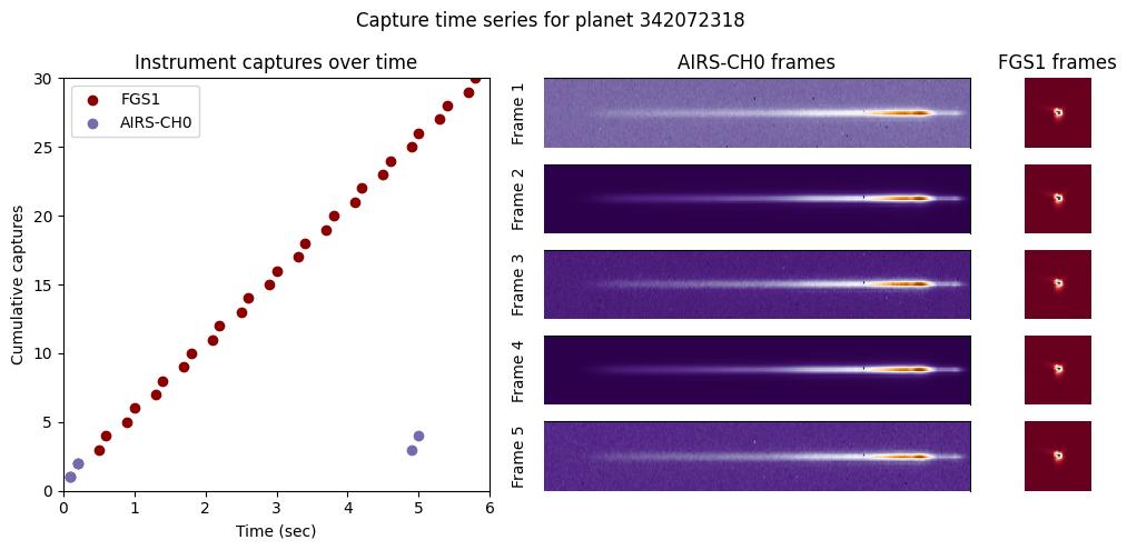
The pattern is clear once you know what to look for. Each instrument takes paired exposures:
- FGS1: Short (0.1s) + long (0.2s) exposures every ~0.5 seconds
- AIRS-CH0: Short (0.1s) + long (4.5s) exposures every ~5 seconds
The timing is deliberately offset so that the “short” exposure ends just before the “long” exposure begins. This CDS approach helps reduce read noise by subtracting the paired frames.
3. Implementing CDS recovery
The key insight from the timing analysis: subtract the second (long) exposure from the first (short) exposure to get the cleaned signal. This halves the number of frames but should significantly reduce noise.
Testing this on a sample planet:
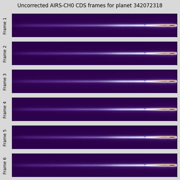
AIRS-CH0 CDS frames
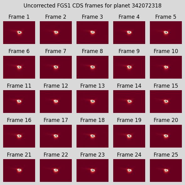
FGS1 CDS frames
The CDS processing works - we get positive signal values and the frame count is exactly halved. However, CDS is just one step in the full calibration pipeline.
4. TODO: image correction/calibration
This is only one step in the basic data preprocessing pipeline - proper data reduction is going to be crucial. The complete preprocessing pipeline needs to handle:
- Analog-to-Digital Conversion - Convert raw counts to physical units
- Hot/Dead Pixel Masking - Remove problematic detector pixels
- Linearity Correction - Account for non-linear detector response
- Dark Current Subtraction - Remove thermal background
- Correlated Double Sampling - Reduce read noise (what we just implemented)
- Flat Field Correction - Normalize pixel-to-pixel sensitivity
CDS alone isn’t enough - we need the full treatment to get clean, calibrated data suitable for exoplanet analysis.
5. Next Steps
With the timing structure decoded and CDS implemented, the next priority is building out the complete signal correction pipeline. The raw data is definitely there, but it needs serious cleanup before we can reliably extract planetary spectra.
The good news: the instruments are well-synchronized and the CDS strategy is working as designed. The challenge now is implementing the remaining calibration steps to turn detector outputs into science-ready data.