Statistics Overview
Statistics is the foundation of data science, providing the mathematical framework for analyzing data, quantifying uncertainty, and making informed decisions. This guide covers essential descriptive statistics, probability distributions, and hypothesis testing methods used in data analysis.
Table of Contents
1. Common Descriptive Statistics
Descriptive statistics summarize and describe the main features of a dataset. They are divided into three main categories based on what aspect of the data they measure.
1.1. Measures of Central Tendency, Spread, and Shape
| Category | Statistic | Description | Formula / Calculation | When to Use | Python Implementation |
|---|---|---|---|---|---|
| Central Tendency | Mean (μ or x̄) | Average of all values; sum divided by count | μ = Σx / n | Symmetric distributions without outliers | np.mean(data) or data.mean() |
| Median | Middle value when data is ordered; 50th percentile | Middle value or average of two middle values | Skewed distributions or data with outliers | np.median(data) or data.median() |
|
| Mode | Most frequently occurring value(s) | Value with highest frequency | Categorical data or multimodal distributions | statistics.mode(data) or data.mode() |
|
| Trimmed Mean | Mean after removing extreme values (e.g., top/bottom 5%) | Mean of remaining values after trimming | Data with outliers but want mean-like measure | scipy.stats.trim_mean(data, 0.05) |
|
| Spread | Range | Difference between maximum and minimum values | Range = max - min | Quick measure of spread; sensitive to outliers | np.ptp(data) or max(data) - min(data) |
| Variance (σ² or s²) | Average squared deviation from the mean | σ² = Σ(x - μ)² / n | Understanding variability; basis for other stats | np.var(data) or data.var() |
|
| Standard Deviation (σ or s) | Square root of variance; typical distance from mean | σ = √(Σ(x - μ)² / n) | Most common spread measure; same units as data | np.std(data) or data.std() |
|
| Interquartile Range (IQR) | Difference between 75th and 25th percentiles | IQR = Q3 - Q1 | Robust to outliers; used in boxplots | scipy.stats.iqr(data) or data.quantile(0.75) - data.quantile(0.25) |
|
| Mean Absolute Deviation (MAD) | Average absolute deviation from the mean | MAD = Σ|x - μ| / n | Less sensitive to outliers than variance | np.mean(np.abs(data - np.mean(data))) |
|
| Coefficient of Variation (CV) | Relative standard deviation (standardized measure) | CV = (σ / μ) × 100% | Comparing variability across different scales | (np.std(data) / np.mean(data)) * 100 |
|
| Shape | Skewness | Measure of asymmetry in the distribution | Positive: right tail; Negative: left tail; 0: symmetric | Assessing distribution symmetry | scipy.stats.skew(data) or data.skew() |
| Kurtosis | Measure of tailedness (outlier propensity) | Positive: heavy tails; Negative: light tails; 0: normal | Identifying presence of outliers | scipy.stats.kurtosis(data) or data.kurtosis() |
1.2. Interpretation Guidelines
Central Tendency
- Mean = Median = Mode: Perfectly symmetric distribution
- Mean > Median: Right-skewed (positive skew) distribution
- Mean < Median: Left-skewed (negative skew) distribution
Spread
- Low variance/SD: Data points cluster closely around the mean
- High variance/SD: Data points are widely dispersed
- IQR: Contains the middle 50% of the data
- CV < 15%: Low variability; CV > 30%: High variability
Shape
- Skewness:
- Between -0.5 and 0.5: Approximately symmetric
- Between -1 and -0.5 or 0.5 and 1: Moderately skewed
- Less than -1 or greater than 1: Highly skewed
- Kurtosis (Excess Kurtosis):
- Approximately 0: Normal distribution
- Greater than 0: Heavy tails, more outliers
- Less than 0: Light tails, fewer outliers
1.3. Choosing the Right Statistic
- For symmetric data without outliers: Use mean and standard deviation
- For skewed data or data with outliers: Use median and IQR
- For comparing variability across different scales: Use coefficient of variation
- For understanding distribution shape: Calculate skewness and kurtosis
- For categorical data: Use mode and frequency tables
1.4. Important Notes
- Always visualize your data (histograms, boxplots, Q-Q plots) before choosing statistics
- Report multiple measures to give a complete picture of your data
- Consider the context and purpose of your analysis when selecting statistics
- Remember that descriptive statistics can be misleading without understanding the underlying distribution
2. Common Probability Distributions
Probability distributions describe the likelihood of different outcomes in a random process. They are fundamental to statistical inference, hypothesis testing, and predictive modeling.
| Type | Distribution | Parameters | Description | Python Implementation | Distribution Shape |
|---|---|---|---|---|---|
| Discrete | Bernoulli | p (probability of success) | Single trial with two outcomes (success/failure) | stats.bernoulli.pmf(k, p) |
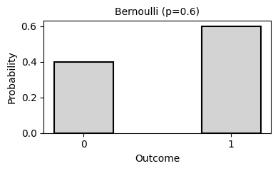 |
| Binomial | n (trials), p (probability) | Number of successes in n independent Bernoulli trials | stats.binom.pmf(k, n, p) |
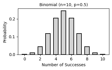 |
|
| Poisson | λ (lambda, rate) | Number of events in fixed time/space interval | stats.poisson.pmf(k, mu) |
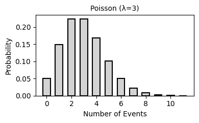 |
|
| Geometric | p (probability of success) | Number of trials until first success | stats.geom.pmf(k, p) |
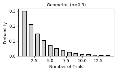 |
|
| Continuous | Uniform | a (min), b (max) | All values in interval [a, b] equally likely | stats.uniform.pdf(x, a, b-a) |
 |
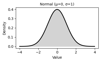
| Normal (Gaussian) | μ (mean), σ (std dev) | Symmetric bell curve; most common distribution | stats.norm.pdf(x, mu, sigma) |
 |
|
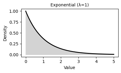
| Exponential | λ (rate) | Time between events in Poisson process | stats.expon.pdf(x, scale=1/lambda) |
 |
|
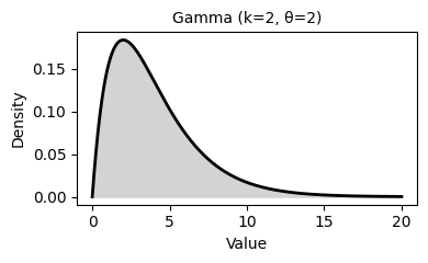
| Gamma | k (shape), θ (scale) | Generalizes exponential; sum of k exponential variables | stats.gamma.pdf(x, k, scale=theta) |
 |
|
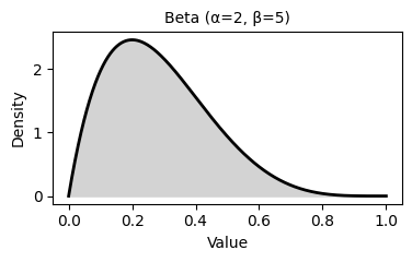
| Beta | α (alpha), β (beta) | Distribution on interval [0, 1] | stats.beta.pdf(x, alpha, beta) |
 |
|
| Chi-Square (χ²) | df (degrees of freedom) | Sum of squared standard normal variables | stats.chi2.pdf(x, df) |
 |
|
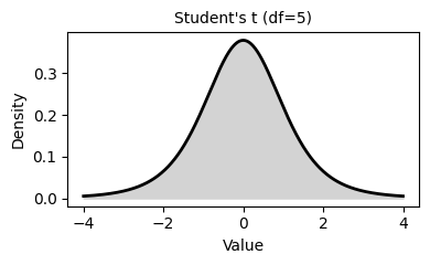
| Student's t | df (degrees of freedom) | Similar to normal but with heavier tails | stats.t.pdf(x, df) |
 |
|
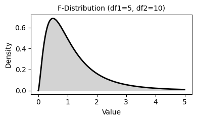
| F-Distribution | df1, df2 (degrees of freedom) | Ratio of two chi-square distributions | stats.f.pdf(x, df1, df2) |
 |
|
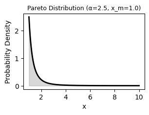
| Pareto | α (shape), xₘ (scale/minimum) | Power law distribution; models 80/20 rule phenomena | stats.pareto.pdf(x, alpha, scale=xm) |
 |
3. Statistical Test Selection Guide
This comprehensive guide helps you choose the appropriate statistical test based on your research question, variable types, and data characteristics.
Note: Parametric tests assume normally distributed data and equal variances, while non-parametric tests make no assumptions about the underlying distribution and are more robust to outliers. A “low p-value” typically means p < 0.05 (or your chosen significance level α).
3.1. Test Assumptions Checklist
Before conducting any statistical test, verify the following assumptions:
Parametric Test Assumptions
- Normality: Data follows a normal distribution
- Shapiro-Wilk test: Best for small to medium samples (n < 5000)
stat, p = stats.shapiro(data)- Low p-value → reject normality assumption
- Kolmogorov-Smirnov test: Better for larger samples, can test against any distribution
stat, p = stats.kstest(data, 'norm', args=(mean, std))- Low p-value → distribution differs from specified distribution
- Q-Q plots: Visual assessment of normality
- Shapiro-Wilk test: Best for small to medium samples (n < 5000)
- Independence: Observations are independent of each other
- Homogeneity of variance: Equal variances across groups (use Levene’s test)
stat, p = stats.levene(group1, group2, group3)
- Sample size: Generally n ≥ 30 for Central Limit Theorem to apply
When to Use Non-Parametric Tests
- Small sample sizes (n < 30)
- Non-normal distributions that cannot be transformed
- Ordinal data or ranks
- Presence of significant outliers
- Violations of parametric test assumptions
3.2. Hypothesis Testing by Scenario
| Independent Variable Type | Dependent Variable Type | Situation | Parametric Test | Non-Parametric Test | P-value Interpretation |
|---|---|---|---|---|---|
| None | Continuous | Comparing one sample to a known value | One-sample T-test / Z-test | Wilcoxon signed-rank test | Low p-value: Sample mean significantly differs from known value |
| Testing normality of data | Shapiro-Wilk test | Kolmogorov-Smirnov test | Low p-value: Data significantly deviates from normal distribution | ||
| Comparing sample distribution to theoretical distribution | N/A | Kolmogorov-Smirnov test | Low p-value: Sample distribution differs from theoretical distribution | ||
| Categorical | Comparing distributions of categorical variables | Chi-square test | Fisher's exact test (for small samples) | Low p-value: Observed distribution differs from expected | |
| Categorical | Continuous | Comparing two independent groups | Independent samples T-test / Two-sample Z-test | Mann-Whitney U test (Wilcoxon rank-sum test) | Low p-value: Significant difference between the two groups |
| Comparing two paired/dependent groups | Paired T-test | Wilcoxon signed-rank test | Low p-value: Significant change between paired observations | ||
| Comparing three or more independent groups | One-way ANOVA | Kruskal-Wallis H test | Low p-value: At least one group differs from the others | ||
| Comparing three or more paired/dependent groups | Repeated measures ANOVA | Friedman test | Low p-value: Significant differences across repeated measurements | ||
| Testing effects of two or more factors | Two-way ANOVA / Factorial ANOVA | Scheirer-Ray-Hare test | Low p-value: Significant main effects or interaction effects | ||
| Comparing variances between two groups | F-test (Levene's test) | Levene's test / Fligner-Killeen test | Low p-value: Variances significantly differ between groups | ||
| Categorical | Testing independence of two categorical variables | Chi-square test of independence | Fisher's exact test | Low p-value: Variables are dependent (not independent) | |
| Continuous | Continuous | Testing relationship between two continuous variables | Pearson correlation | Spearman rank correlation / Kendall's tau | Low p-value: Significant correlation exists between variables |
3.3. Multiple Testing Correction
The Multiple Comparisons Problem
When performing multiple statistical tests simultaneously, the probability of obtaining at least one false positive (Type I error) increases dramatically. This is known as the multiple comparisons problem or multiple testing problem.
Example: If you conduct 20 independent tests at α = 0.05, the probability of at least one false positive is approximately 64%, not 5%!
Why It Matters
- Inflated Type I Error Rate: Each additional test increases the family-wise error rate (FWER)
- False Discoveries: You’re more likely to identify “significant” results that are actually due to chance
- Reproducibility Issues: Results that appear significant may not replicate in future studies
Common Correction Methods
Multiple testing correction methods are available in the multipletests class from the statsmodels.stats.multitest module in the Statsmodels Python library.
- Bonferroni Correction
- Most conservative approach
- Adjusted α = α / number of tests
- Example: For 10 tests at α = 0.05, use α = 0.005 for each test
- Best for: Small number of tests, when minimizing false positives is critical
- Python:
multipletests(pvals, method='bonferroni')
- Holm-Bonferroni (Sequential Bonferroni)
- Less conservative than Bonferroni
- Orders p-values and applies sequential testing
- More powerful while controlling FWER
- Python:
multipletests(pvals, method='holm')
- False Discovery Rate (FDR) - Benjamini-Hochberg
- Controls the proportion of false positives among rejected hypotheses
- Less conservative than Bonferroni
- Best for: Exploratory research, large numbers of tests
- Python:
multipletests(pvals, method='fdr_bh')
- Post-hoc Tests
- Used after ANOVA when comparing specific group pairs
- Methods: Tukey’s HSD, Dunnett’s test, Scheffé’s test
- Built-in corrections for multiple pairwise comparisons
- Python:
from statsmodels.stats.multicomp import pairwise_tukeyhsd
Best Practices
- Plan Ahead: Define your hypotheses before collecting data to minimize unnecessary tests
- Adjust When Needed: Always apply corrections when testing multiple hypotheses in the same dataset
- Report Transparently: Clearly state which correction method (if any) was used
- Consider Context: Balance between Type I and Type II errors based on your research goals
- Use Post-hoc Tests: After ANOVA, use appropriate post-hoc tests rather than multiple t-tests
Remember: Failing to account for multiple testing can lead to spurious findings and undermine the validity of your research conclusions.